Functor and Applicative

In this chapter we see how the Haskell language features we introduced in previous chapters (from function application rules based on Lambda Calculus to Typeclasses) lead to highly flexible and refactorable code and powerful abstractions.

Learning Outcomes

Understand how eta-conversion, operator sectioning and compose, together provide the ability to transform code to achieve a composable point free form and use this technique to refactor code.
Understand that in Haskell the ability to map over container structures is generalised into the Functor typeclass, such that any type that is an instance of Functor has the fmap or (<$>) operation.
Understand that the Applicative Typeclass extends Functor such that containers of functions may be applied (using the (<*>) operator) to containers of values.
Understand that Functor and Applicative allow powerful composable types through exploring a simple applicative functor for parsing.

Refactoring Cheatsheet

The following equivalences make many refactorings possible in Haskell:

Eta Conversion

Exactly as per Lambda Calculus:

 f x ≡ g x
 f   ≡ g

Operator Sectioning

Remember haskell binary operators are just infix curried functions of two parameters and that putting brackets around them makes them prefix instead of infix.

 x + y ≡ (+) x y
       ≡ ((+) x) y  -- making function application precedence explicit
       ≡ (x+) y     -- binary operators can also be partially applied

Such operator sectioning allows us to get the right-most parameter of the function on it’s own at the right-hand side of the body expression such that we can apply Eta conversion, thus:

f x = 1 + x
f x = (1+) x
f = (1+)             -- Eta conversion

Compose

Has its own operator in haskell (.), inspired by the mathematical function composition symbol ∘:

 (f ∘ g) (x) ≡ f (g(x)) -- math notation
 (f . g) x ≡ f (g x)    -- Haskell

Again, this gives us another way to get the right-most parameter on its own outside the body expression:

f x = sqrt (1 / x)
f x = sqrt ((1/) x)     -- operator section
f x = (sqrt . (1/)) x   -- by the definition of composition
f = sqrt . (1/)         -- eta conversion

Point-Free Code

We have discussed point-free and tacit coding style earlier in these notes. In particular, eta-conversion works in Haskell the same as in lambda calculus and for curried JavaScript functions. It is easy to do and usually declutters code of unnecessary arguments, e.g.:

lessThan :: (Ord a) => a -> [a] -> [a]
lessThan n aList = filter (<n) aList

The following is more concise, and once you are used to reading haskell type definitions, just as self evident:

lessThan :: (Ord a) => a -> [a] -> [a]
lessThan n = filter (<n)

But the above still has an argument (a point), n. Can we go further?

It is possible to be more aggressive in refactoring code to achieve point-free style by using the compose operator (.):

(.) :: (b -> c) -> (a -> b) -> a -> c
(f . g) x = f (g x)

To see how to use (.) in lessThan we need to refactor it to look like the right-hand side of the definition above, i.e. f (g x). For lessThan, this takes a couple of steps, because the order we pass arguments to (<) matters. Partially applying infix operators like (<n) is called operator sectioning. Placing n after < means that it is being passed as the second argument to the operator, which is inconvenient for eta-conversion. Observe that (<n) is equivalent to (n>), so the following is equivalent to the definition above:

lessThan n = filter (n>)

Now we can use the non-infix form of (>):

lessThan n = filter ((>) n)

And we see from our definition of compose, that if we were to replace filter by f, (>) by g, and n by x, we would have exactly the definition of (.). Thus,

lessThan n = (filter . (>)) n

And now we can apply eta-conversion:

lessThan = filter . (>)

Between operator sectioning, the compose combinator (.), and eta-conversion it is possible to write many functions in point-free form. For example, the flip combinator:

flip :: (a -> b -> c) -> b -> a -> c
flip f a b = f b a

can also be useful in reversing the arguments of a function or operator in order to get them into a position such that they can be eta-reduced.

In code written by experienced haskellers it is very common to see functions reduced to point-free form. Does it make code more readable? To experienced haskellers, many times yes. To novices, perhaps not. When to do it is a matter of preference. Experienced haskellers tend to prefer it, they will argue that it reduces functions like the example one above “to their essence”, removing the “unnecessary plumbing” of explicitly named variables. Whether you like it or not, it is worth being familiar with the tricks above, because you will undoubtedly see them used in practice. The other place where point-free style is very useful is when you would otherwise need to use a lambda function.

Some more (and deeper) discussion is available on the Haskell Wiki.

Exercises

Refactor the following function to be point-free:

f a b c = (a+b)*c

(This is clearly an extreme example but is a useful – and easily verified – practice of operator sectioning, composition and eta-conversion.)

Functor

We’ve been mapping over lists and arrays many times, first in JavaScript:

console> [1,2,3].map(x=>x+1)
[2,3,4]

Now in Haskell:

GHCi> map (\i->i+1) [1,2,3]
[2,3,4]

Or (eta-reduce the lambda to be point-free):

GHCi> map (+1) [1,2,3]
[2,3,4]

Here’s the implementation of map for lists as it’s defined in the GHC standard library:

map :: (a -> b) -> [a] -> [b]
map _ []     = []
map f (x:xs) = f x : map f xs

It’s easy to generalise this pattern to any data structure that holds one or more values: mapping a function over a data structure creates a new data structure whose elements are the result of applying the function to the elements of the original data structure.

In Haskell this pattern is captured in a type class called Functor, which defines a function called fmap.

Prelude> :i Functor
type Functor :: (* -> *) -> Constraint
class Functor f where
  fmap :: (a -> b) -> f a -> f b
...
instance Functor [] -- naturally lists are an instance
instance Functor Maybe -- but this may surprise!
... -- and some other instances we'll talk about shortly

The first line says that an instances of the Functor typeclass f must be over a type that has the kind (* -> *), that is, their constructors must be parameterised with a single type variable. After this, the class definition specifies fmap as a function that will be available to any instance of Functor and that f is the type parameter for the constructor function, which again, takes one type parameter, e.g. f a as the input to fmap, which returns an f b.

Naturally, lists have an instance:

Prelude> :i []
...
instance Functor [] -- Defined in `GHC.Base'

We can actually look up GHC’s implementation of fmap for lists and we see:

instance Functor [] where
    fmap = map

And here’s the instance for Maybe:

instance  Functor Maybe  where
    fmap _ Nothing       = Nothing
    fmap f (Just a)      = Just (f a)

So we can fmap a function over a Maybe without having to unpack it:

GHCi> fmap (+1) (Just 6)
Just 7 

This is such a common operation that there is an operator alias for fmap: <$>

GHCi> (+1) <$> (Just 6)
Just 7 

Which also works over lists:

GHCi> (+1) <$> [1,2,3]
[2,3,4] 

Lists of Maybes frequently arise. For example, the mod operation on integers (e.g. mod 3 2 == 1) will throw an error if you pass 0 as the divisor:

> mod 3 0
*** Exception: divide by zero 

We might define a safe modulo function:

safeMod :: Integral a => a-> a-> Maybe a
safeMod _ 0 = Nothing
safeMod numerator divisor = Just $ mod numerator divisor 

This makes it safe to apply safeMod to an arbitrary list of Integral values:

> map (safeMod 3) [1,2,0,4]
[Just 0,Just 1,Nothing,Just 3] 

But how do we keep working with such a list of Maybes? We can map an fmap over the list:

GHCi> map ((+1) <$>) [Just 0,Just 1,Nothing,Just 3]
[Just 1,Just 2,Nothing,Just 4] 

Or equivalently:

GHCi> ((+1) <$>) <$> [Just 0,Just 1,Nothing,Just 3]
[Just 1,Just 2,Nothing,Just 4] 

In addition to lists and Maybes, a number of other built-in types have instances of Functor:

GHCi> :i Functor
...
instance Functor (Either a) -- Defined in `Data.Either'
instance Functor IO -- Defined in `GHC.Base'
instance Functor ((->) r) -- Defined in `GHC.Base'
instance Functor ((,) a) -- Defined in `GHC.Base' 

The definition for functions (->) might surprise:

instance Functor ((->) r) where
    fmap = (.) 

So the composition of functions f and g, f . g, is equivalent to ‘mapping’ f over g, e.g. f <$> g.

GHCi> f = (+1)
GHCi> g = (*2)
GHCi> (f.g) 3
7
GHCi> (f<$>g) 3
7

Functor Laws

We can formalise the definition of Functor with two laws:

The law of identity

∀ x: (id <$> x) ≡ x

The law of composition

∀ f, g, x: (f ∘ g <$> x) ≡ (f <$> (g <$> x))

Note that these laws are not enforced by the compiler when you create your own instances of Functor. You’ll need to test them for yourself. Following these laws guarantees that general code (e.g. algorithms) using fmap will also work for your own instances of Functor.

Let’s make a custom instance of Functor for a simple binary tree type and check that the laws hold. Here’s a simple binary tree datatype:

data Tree a = Empty
            | Leaf a
            | Node (Tree a) a (Tree a)
  deriving (Show)

Note that Leaf is a bit redundant as we could also encode nodes with no children as Node Empty value Empty – but that’s kind of ugly and makes showing our trees more verbose. Also, having both Leaf and Empty provides a nice parallel to Maybe.

Here’s an example tree defined:

tree = Node (Node (Leaf 1) 2 (Leaf 3)) 4 (Node (Leaf 5) 6 (Leaf 7))

And here’s a visualisation of the tree:

Node 4
 ├──Node 2
 |   ├──Leaf 1
 |   └──Leaf 3
 └──Node 6
     ├──Leaf 5
     └──Leaf 7

And here’s the instance of Functor for Tree that defines fmap.

instance Functor Tree where
   fmap :: (a -> b) -> Tree a -> Tree b
   fmap _ Empty = Empty
   fmap f (Leaf v) = Leaf $ f v
   fmap f (Node l v r) = Node (fmap f l) (f v) (fmap f r)

Just as in the Maybe instance above, we use pattern matching to define a case for each possible constructor in the ADT. The Empty and Leaf cases are very similar to Maybe fmap for Nothing and Just respectively, that is, for Empty we just return another Empty, for Leaf we return a new Leaf containing the application of f to the value x stored in the leaf. The fun one is Node. As for Leaf, fmap f of a Node returns a new Node whose own value is the result of applying f to the value stored in the input Node, but the left and right children of the new node will be the recursive application of fmap f to the children of the input node.

Now we’ll demonstrate (but not prove) that the two laws hold at least for our example tree:

Law of Identity:

> id <$> tree
Node (Node (Leaf 1) 2 (Leaf 3)) 4 (Node (Leaf 5) 6 (Leaf 7))

Law of Composition:

> (+1) <$> (*2) <$> tree
Node (Node (Leaf 3) 5 (Leaf 7)) 9 (Node (Leaf 11) 13 (Leaf 15))
> (+1).(*2) <$> tree
Node (Node (Leaf 3) 5 (Leaf 7)) 9 (Node (Leaf 11) 13 (Leaf 15))

Applicative

The typeclass Applicative introduces a new operator <*> (pronounced “apply”), which lets us apply functions inside a computational context.

Applicative is a “subclass” of Functor, meaning that an instance of Applicative can be fmaped over, but Applicatives also declare (at least) two additional functions, pure and (<*>) (pronounced ‘apply’ – but I like calling it “TIE Fighter”):

GHCi> :i Applicative
class Functor f => Applicative (f :: * -> *) where
  pure :: a -> f a
  (<*>) :: f (a -> b) -> f a -> f b
...

As for Functor all instances of the Applicative type-class must satisfy certain laws, which again are not checked by the compiler. Applicative instances must comply with these laws to produce the expected behaviour. You can read about the Applicative Laws if you are interested, but they are a little more subtle than the basic Functor laws above, and it is not essential to understand them to be able to use <*> in Haskell.

As for Functor, many Base Haskell types are also Applicative, e.g. [], Maybe, IO and (->).

For example, a function inside a Maybe can be applied to a value in a Maybe.

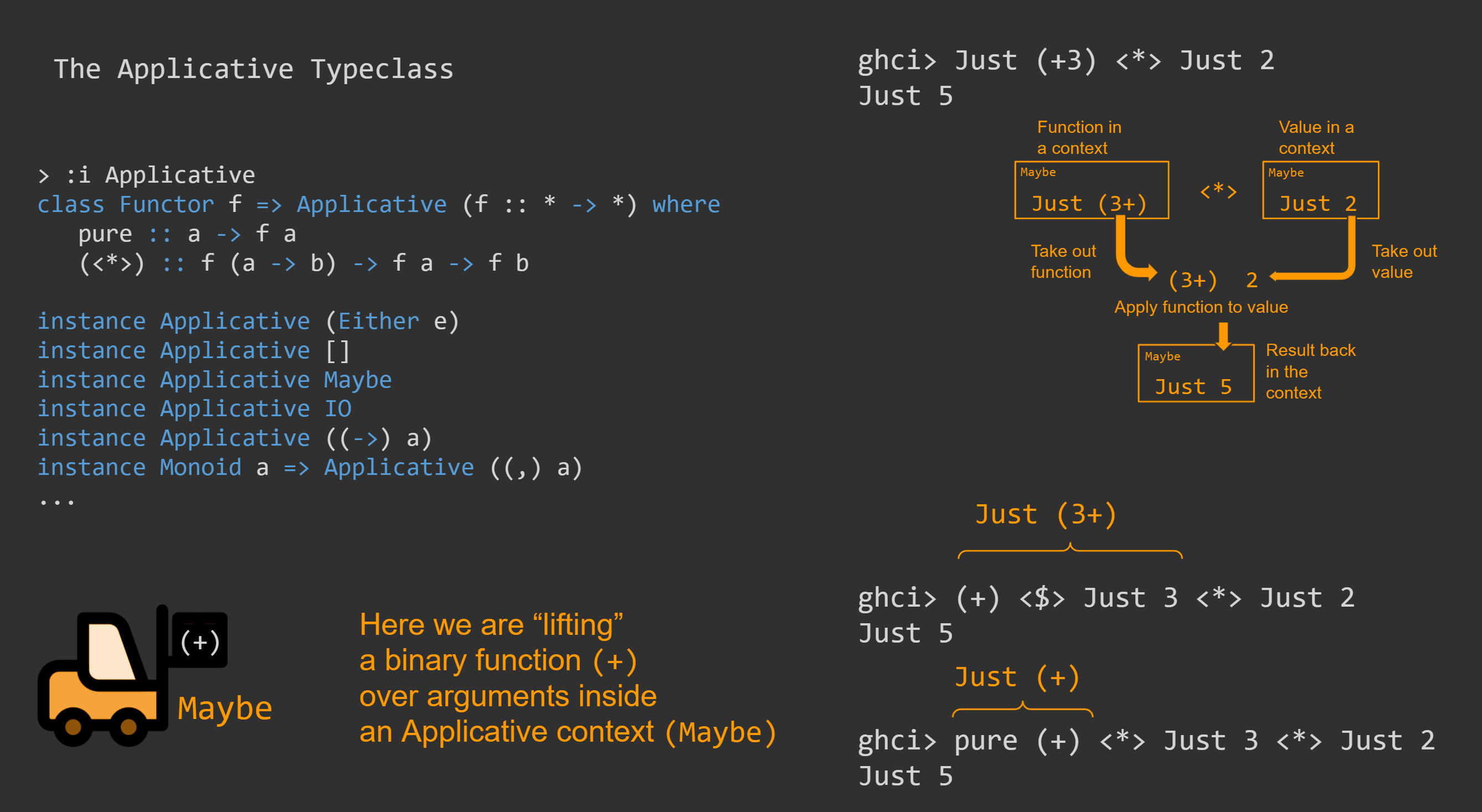
GHCi> Just (+3) <*> Just 2
Just 5 

Or a list of functions [(+1),(+2)] to things inside a similar context (e.g. a list [1,2,3]).

> [(+1),(+2)] <*> [1,2,3]
[2,3,4,3,4,5] 

Note that lists definition of <*> produces the Cartesian product of the two lists, that is, all the possible ways to apply the functions in the left list to the values in the right list. It is interesting to look at the source for the definition of Applicative for lists on Hackage:

instance Applicative [] where
  pure x    = [x]
  fs <*> xs = [f x | f <- fs, x <- xs]  -- list comprehension 

The definition of <*> for lists uses a list comprehension. List comprehensions are a short-hand way to generate lists, using notation similar to mathematical “set builder notation”. The set builder notation here would be: {f(x) | f ∈ fs ∧ x ∈ xs}. In English it means: “the set (Haskell list) of all functions in fs applied to all values in xs”.

A common use-case for Applicative is applying a binary (two-parameter) function over two Applicative values, e.g.:

> pure (+) <*> Just 3 <*> Just 2
Just 5 

So:

pure puts the binary function into the applicative (i.e. pure (+) :: Maybe (Num -> Num -> Num)),
then <*>ing this function inside over the first Maybe value Just 3 achieves a partial application of the function inside the Maybe. This gives a unary function inside a Maybe: i.e. Just (3+) :: Maybe (Num->Num).
Finally, we <*> this function inside a Maybe over the remaining Maybe value.

This is where the name “applicative” comes from, i.e. Applicative is a type over which a non-unary function may be applied. Note, that the following use of <$> (infix fmap) is equivalent and a little bit more concise:

> (+) <$> Just 3 <*> Just 2
Just 5 

This is also called “lifting” a function over an Applicative. Actually, it’s so common that Applicative also defines dedicated functions for lifting binary functions (in the GHC.Base module):

> GHC.Base.liftA2 (+) (Just 3) (Just 2)
Just 5 

Here’s a little visual summary of Applicative and lifting (box metaphor inspired by adit.io):

Applicative Visual Summary

It’s also useful to lift binary data constructors over two Applicative values, e.g. for tuples:

> (,) <$> Just 3 <*> Just 2
Just (3, 2) 

We can equally well apply functions with more than two arguments over the correct number of values inside Applicative contexts. Recall our student data type:

data Student = Student { id::Integer, name::String, mark::Int } 

with a ternary constructor:

Student::Integer -> String -> Int -> Student

Let’s say we want to create a student for a given id but we need to look up the name and mark from tables, i.e. lists of key-value pairs: names::[(Integer,String)] and marks::[(Integer,Int)]. We’ll use the function lookup :: Eq a => a -> [(a, b)] -> Maybe b, which will either succeed with Just the result, or fail to find the value for a given key, and return Nothing.

lookupStudent :: Integer -> Maybe Student
lookupStudent sid = Student sid <$> lookup sid names <*> lookup sid marks

Lists are also instances of Applicative. Given the following types:

data Suit = Spade|Club|Diamond|Heart
 deriving (Eq,Ord,Enum,Bounded)

instance Show Suit where
 show Spade = "^"     -- ♠	 (closest I could come in ASCII was ^)
 show Club = "&"      -- ♣
 show Diamond = "O"   -- ♦
 show Heart = "V"     -- ♥

data Rank = Two|Three|Four|Five|Six|Seven|Eight|Nine|Ten|Jack|Queen|King|Ace
 deriving (Eq,Ord,Enum,Show,Bounded)

data Card = Card Suit Rank
 deriving (Eq, Ord, Show) 

We can make one card using the Card constructor:

GHCi> Card Spade Ace
Card ^ Ace 

Or, since both Suit and Rank derive Enum, we can enumerate the full lists of Suits and Ranks, and then lift the Card operator over both lists to create a whole deck:

GHCi> Card <$> [Spade ..] <*> [Two ..]
[Card ^ Two,Card ^ Three,Card ^ Four,Card ^ Five,Card ^ Six,Card ^ Seven,Card ^ Eight,Card ^ Nine,Card ^ Ten,Card ^ Jack,Card ^ Queen,Card ^ King,Card ^ Ace,Card & Two,Card & Three,Card & Four,Card & Five,Card & Six,Card & Seven,Card & Eight,Card & Nine,Card & Ten,Card & Jack,Card & Queen,Card & King,Card & Ace,Card O Two,Card O Three,Card O Four,Card O Five,Card O Six,Card O Seven,Card O Eight,Card O Nine,Card O Ten,Card O Jack,Card O Queen,Card O King,Card O Ace,Card V Two,Card V Three,Card V Four,Card V Five,Card V Six,Card V Seven,Card V Eight,Card V Nine,Card V Ten,Card V Jack,Card V Queen,Card V King,Card V Ace] 

Exercise

Create instances of Show for Rank and Card such that a deck of cards displays much more succinctly, e.g.:

[^2,^3,^4,^5,^6,^7,^8,^9,^10,^J,^Q,^K,^A,&2,&3,&4,&5,&6,&7,&8,&9,&10,&J,&Q,&K,&A,O2,O3,O4,O5,O6,O7,O8,O9,O10,OJ,OQ,OK,OA,V2,V3,V4,V5,V6,V7,V8,V9,V10,VJ,VQ,VK,VA]

Try and make the definition of show for Rank a one-liner using zip and lookup.

Different Ways To Apply Functions Cheatsheet

 g x         -- apply function g to argument x
 g $ x       -- apply function g to argument x
 g <$> f x   -- apply function g to argument x which is inside Functor f
 f g <*> f x -- apply function g in Applicative context f to argument x which is also inside f

We saw that functions (->) are Functors, such that (<$>)=(.). There is also an instance of Applicative for functions of input type r. We’ll give the types of the essential functions for the instance:

instance Applicative ((->)r) where
  pure :: a -> (r->a)
  (<*>) :: (r -> (a -> b)) -> (r -> a) -> (r -> b)

This is very convenient for creating point-free implementations of functions which operate on their parameters more than once. For example, imagine our Student type from above has additional fields with breakdowns of marks: e.g. exam and nonExam, requiring a function to compute the total mark:

totalMark :: Student -> Int
totalMark s = exam s + nonExam s

Here’s the point-free version, taking advantage of the fact that exam and nonExam, both being functions of the same input type Student, are both in the same Applicative context:

totalMark = (+) <$> exam <*> nonExam

Or equivalently:

totalMark = (+) . exam <*> nonExam

Exercise

derive the implementations of pure and <*> for Maybe and for functions ((->)r).

(hint, if you get stuck there are spoilers in the source from GHC.Base that I linked above)

Alternative

The Alternative typeclass is another important typeclass in Haskell, which is closely related to the Applicative typeclass. It introduces a set of operators and functions that are particularly useful when dealing with computations that can fail or have multiple possible outcomes. Alternative is also considered a “subclass” of Applicative, and it provides additional capabilities beyond what Applicative offers. It introduces two main functions, empty and <|> (pronounced “alt” or “alternative”)

class Applicative f => Alternative (f :: * -> *) where
  empty :: f a
  (<|>) :: f a -> f a -> f a

empty: This function represents a computation with no result or a failure. It serves as the identity element. For different data types that are instances of Alternative, empty represents an empty container or a failed computation, depending on the context.

(<|>): The <|> operator combines two computations, and it’s used to express alternatives. It takes two computations of the same type and returns a computation that will produce a result from the first computation if it succeeds, or if it fails, it will produce a result from the second computation. This operator allows you to handle branching logic and alternative paths in your code.

Like Functor and Applicative, instances of the Alternative typeclass must also adhere to specific laws, ensuring predictable behavior when working with alternatives. Common instances of the Alternative typeclass include Maybe and lists ([]). Alternatives are also very useful for Parsers, where we try to run first parser, if it fails, we run the second parser.

> Just 2 <|> Just 5
Just 2

> Nothing <|> Just 5
Just 5

A simple Applicative Functor for Parsing

As we will discuss in more detail later, a parser is a program which takes some structured input and does something with it. When we say “structured input” we typically mean something like a string that follows strict rules about its syntax, like source code in a particular programming language, or a file format like JSON. A parser for a given syntax is a program which you run over some input and if the input is valid, it will do something sensible with it (like give us back some data), or fail: preferably in a way that we can handle gracefully.

In Haskell, sophisticated parsers are often constructed from simple functions which try to read a certain element of the expected input and either succeed in consuming that input, returning a tuple containing the rest of the input string and the resultant data, or they fail producing nothing. We’ve already seen one type which can be used to encode success or failure, namely Maybe. Here’s the most trivial parser function I can think of. It tries to take a character from the input stream and either succeeds consuming it or fails if it’s given an empty string:

-- >>> parseChar "abc"
-- Just ("bc",'a')
-- >>> parseChar ""
-- Nothing
parseChar :: String -> Maybe (String, Char)
parseChar "" = Nothing
parseChar (c:rest) = Just (rest, c)

And here’s one to parse Ints off the input stream. It uses the reads function from the Prelude:

-- >>> parseInt "123+456"
-- Just ("+456",123)
-- >>> parseInt "xyz456"
-- Nothing
parseInt :: String -> Maybe (String, Int) 
parseInt s = case reads s of     
  [(x, rest)] -> Just (rest, x)
  _           -> Nothing

So now we could combine these to try to build a little calculator language (OK, all it can do is add two integers, but you get the idea):

-- >>> parsePlus "123+456"
-- Just ("",579)
parsePlus :: String -> Maybe (String, Int)
parsePlus s =
    case parseInt s of
        Just (s', x) -> case parseChar s' of
            Just (s'', '+') -> case parseInt s'' of
                Just (s''',y) -> Just (s''',x+y)
                Nothing -> Nothing
            Nothing -> Nothing
        Nothing -> Nothing

But that’s not very elegant and Haskell is all about elegant simplicity. So how can we use Haskell’s typeclass system to make parsers that are more easily combined? We’ve seen how things that are instances of the Functor and Applicative typeclasses can be combined – so let’s make a type definition for parsers and then make it an instance of Functor and Applicative. Here’s a generic type for parsers:

newtype Parser a = Parser (String -> Maybe (String, a))

We can now make concrete parsers for Int and Char using our previous functions:

char :: Parser Char
char = Parser parseChar
int :: Parser Int
int = Parser parseInt

And here’s a generic function we can use to run these parsers:

-- >>> parse int "123+456"
-- Just ("+456",123)
parse :: Parser a -> String -> Maybe (String, a)
parse (Parser p) = p

And here’s a little parser which asserts the next character on the stream is the one we are expecting:

-- >>> parse (is '+') "+456"
-- Just ("456",'+')
-- >>> parse (is '-') "+456"
-- Nothing
is :: Char -> Parser Char
is c = Parser $
  \inputString -> case parse char inputString of
    Just (rest, result) | result == c -> Just (rest, result)
    _ -> Nothing

By making Parser an instance of Functor we will be able to map functions over the result of a parse. The fmap function for the Functor instance of Parser needs to apply the parser to an input string and apply the given function to the result of the parse, i.e.:

instance Functor Parser where
  fmap f (Parser p) = Parser $ 
    \i -> case p i of 
      Just (rest, result) -> Just (rest, f result)
      _ -> Nothing

That definition should not be too difficult to understand. We apply the parser and if it succeeds (returns a Just) we apply the function f to the result.

However, we can take advantage of the fact that the Tuple returned by the parse function is also an instance of Functor to make the definition more succinct. That is, we are applying the function f to the second item of a tuple – that is exactly what the fmap for the Functor instance of a Tuple does! So we can rewrite to use the Tuple fmap, or rather its alias (<$>):

instance Functor Parser where
  fmap f (Parser p) = Parser $ 
    \i -> case p i of 
      Just (rest, result) -> Just (f <$> (rest, result))
      _ -> Nothing

Carefully examining this, what we are doing is applying (f <$>) if the result is a Just, or ignoring if the result is Nothing. This is exactly what the Maybe instance of Functor does, so we can fmap over the Maybe also:

instance Functor Parser where
  fmap f (Parser p) = Parser (\i -> (f <$>) <$> p i )

Let’s try rearrange to make it point point-free, eliminating the lambda: First, let’s add some brackets, to make the evaluation order more explicit.

instance Functor Parser where
  fmap f (Parser p) = Parser (\i -> ((f <$>) <$>) (p i))

This is now in the form (f . g) i) where f is equal to ((f <$>) <$>) and g is equal to p. Therefore:

instance Functor Parser where
  fmap f (Parser p) = Parser (\i -> (((f <$>) <$>) . p) i)

And, if we eta-reduce:

instance Functor Parser where
  fmap f (Parser p) = Parser (((f <$>) <$>) . p)

The last thing we notice is that the Functor instance for functions is defined as compose. Therefore, we have finally reached the end of our journey and can re-write this as follows.

-- >>> parse ((*2) <$> int) "123+456"
-- Just ("+456",246)
instance Functor Parser where
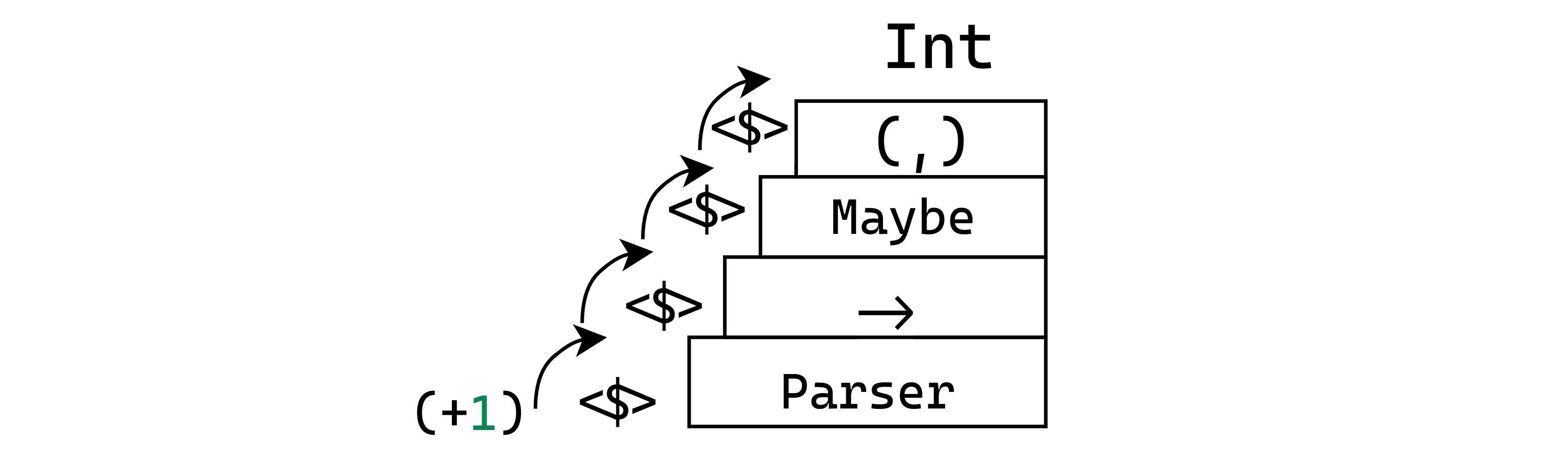
  fmap f (Parser p) = Parser (((f <$>) <$>) <$> p)

The whacky triple-nested application of <$> comes about because the result type a in our Parser type is nested inside a Tuple ((,a)), nested inside a Maybe, nested inside function (->r). So now we can map (or fmap, to be precise) a function over the value produced by a Parser. For example:

> parse ((+1)<$>int) "1bc"
Just ("bc",2)

So (+1)<$>int creates a new Parser which parses an int from the input stream and adds one to the value parsed (if it succeeds). Behind the scenes, using the implementation above, the Parser’s instance of Functor is effectively lifting over three additional layers of nested types to reach the Int value, i.e.:

Applicative Visual Summary

Just as we have seen before, making our Parser an instance of Applicative is going to let us do nifty things like lifting a binary function over the results of two Parsers. Thus, instead of implementing all the messy logic of connecting two Parsers to make plus above, we’ll be able to lift (+) over two Parsers.

Now the definition for the Applicative is going to stitch together all the messy bits of handling both the Just and Nothing cases of the Maybe that we saw above in the definition of plus, abstracting it out so that people implementing parsers like plus won’t have to:

instance Applicative Parser where
  pure a = Parser (\b -> Just (b, a))

  (Parser f) <*> (Parser g) = Parser $ 
    \i -> case f i of                                       -- note that this is just
      Just (r1, p1) -> case g r1 of                         -- an abstraction of the
        Just (r2, p2) -> Just (r2, p1 p2)                   -- logic we saw in `plus`
        Nothing       -> Nothing
      Nothing -> Nothing

All that pure does is put the given value on the right side of the tuple.

The key insight for this applicative instance is that we first use f (the parser on the LHS of <*>). This consumes input from i giving back the remaining input in r1. We then run the second parser g on the RHS of <*> on r1 (the remaining input).

The main take-away message is that <*> allows us to combine two parsers in sequence, that is, we can run the first one and then the second one.

Let’s walk through a concrete example of this.

> charIntPairParser = (,) <$> char <*> int
> parse charIntPairParser "a12345b"
Just ("b",('a',12345))

As both <$> and <*> have the same precedence, firstly (,) <$> char will be evaluated, the result will be then applied to int.

So how does (,) <$> char work? Well, we parse a character and then make that character the first item of a tuple, therefore:

> charPairParser = (,) <$> char
> :t charPairParser
charPairParser :: Parser (b -> (Char, b))

So for the applicative instance the LHS will be the charPairParser and the RHS will be int. That is, first step in applicative parsing is to parse the input i using the LHS parser, what we called here charPairParser. This will match the Just (r1, p1) case where it will be equal to Just ("12345b", ('a',)). Therefore, r1 is equal to the unparsed portion of the input 12345b and the result is a tuple partially applied ('a', ).

We then run the second parser int on the remaining input "12345b". This will match the Just (r2, p2) case where it will be equal to Just ("b", 12345), where r2 is equal to the remaining input "b" and p2 is equal to "12345"

We then return Just (r2, p1 p2), which will evaluate to Just ("b", ('a',12345)).

Using the <*> operator we can make our calculator magnificently simple:

-- >>> parse plus "123+456"
-- Just ("",579)
plus :: Parser Int
plus = (+) <$> int <*> (is '+' *> int)

Note that we make use of a different version of the applicative operator here: *>. Note also that we didn’t have to provide an implementation of *> - rather, the typeclass system picks up a default implementation of this operator (and a bunch of other functions too) from the base definition of Applicative. These default implementations are able to make use of the <*> that we provided for our instance of Applicative for Parser.

Prelude> :t (*>)                        
(*>) :: Applicative f => f a -> f b -> f b

So compared to <*> which took a function inside the Applicative as its first parameter which is applied to the value inside the Applicative of its second parameter, the *> carries through the effect of the first Applicative, but doesn’t do anything else with the value. You can think of it as a simple chaining of effectful operations: “do the first effectful thing, then do the second effectful thing, but give back the result of the second thing only”.

In the context of the Parser instance when we do things like (is '+' *> int), we try the is. If it succeeds then we carry on and run the int. But if the is fails, execution is short circuited and we return Nothing. There is also a flipped version of the operator which works the other way:

Prelude> :t (<*)                        
(<*) :: Applicative f => f a -> f b -> f a

So we could have just as easily implement the plus parser:

-- >>> parse plus "123+456"
-- Just ("",579)
plus :: Parser Int
plus = (+) <$> int <* is '+'  <*> int

Obviously, the above is not a fully featured parsing system. A real parser would need to give us more information in the case of failure, so a Maybe is not really a sufficiently rich type to package the result. Also, a real language would need to be able to handle alternatives - e.g. minus or plus, as well as expressions with an arbitrary number of terms. We will revisit all of these topics with a more feature rich set of parser combinators later.